If you're reading this post and putting together the date and my bio, you've probably already figured out where I work.
Over the past four years spent on the A1 between Milan and Bologna, I've learned a lot and reached some important milestones. The most significant one, accelerated by an AI-driven era, came in the last few months.
I'm referring to the design of a copyright infringement system.
Built as a decision-support tool for its users and powered by the world's largest lyrics catalog, it helps prevent AI systems from generating musical melodies based on copyrighted lyrics.
My mantra has always been that "copyright infringement is decided in court" and as interesting as the topic is, I won't go into the technical details of the current implementation (you would have liked that, though).
That said, what I want to share is one of the explorations I did in my spare time.
Spoiler: Salvatore Sanfilippo AKA @antirez was a major source of inspiration and his name isn't here by accident.
When we talk about song lyrics, we're talking about text. And one of the signals we can look at when reasoning about copyright infringement is pretty simple. Putting the nuances aside for a moment, a basic signal is when the input text used to generate a new melody is partially or fully identical to a copyrighted lyrics.
Text similarity is not a new problem in computer science. It has been addressed by many algorithms over time, each fitting the problem space with different trade-offs.
One of the simplest is Jaccard similarity, defined as the size of the intersection between two documents divided by the size of their union. Essentially, it measures the number of shared words over the total number of unique words across both texts.
It produces a score between 0 and 1: 0 means the documents have nothing in common, while 1 means they are identical.
We can define Jaccard similarity as:
j(doc_1, doc_2) = (doc_1 ∩ doc_2) / (doc_1 ∪ doc_2)
Let's take a simple example:
doc_1 = "Data is the new oil of the digital economy"
doc_2 = "Data is a new oil"
After tokenizing into words:
words_doc1 = {'data', 'is', 'the', 'new', 'oil', 'of', 'digital', 'economy'}
words_doc2 = {'data', 'is', 'a', 'new', 'oil'}
The intersection and union become:
intersection = {'data', 'is', 'new', 'oil'}
union = {'data', 'a', 'of', 'is', 'economy', 'the', 'new', 'digital', 'oil'}
So the final score is:
j(doc_1, doc_2) = 4 / 9 = 0.444
The time complexity of Jaccard similarity is O(n + m), where n and m are the number of words in the two documents.
In practice, it only requires building two hash-based sets and then computing their intersection and union. Once the words are in sets, both operations are linear in the size of the inputs.
Another algorithm, complementary to Jaccard similarity, is the Levenshtein distance.
Jaccard focuses on overlap between sets of elements and doesn't care about order. Levenshtein, on the other hand, measures how many edits (insertions, deletions, substitutions) are needed to transform one sequence into another. It's commonly applied at character level, but it works at any granularity. In fact, applied at word level it becomes the basis for Word Error Rate, a standard metric in speech recognition.
Transforming doc_2 into doc_1 using word-level edits:
- 1 substitution:
a→the - 4 insertions:
of,the,digital,economy
lev(doc_1, doc_2) = 5
To normalize it into a 0–1 range (closer to Jaccard-style intuition):
norm_lev = 1 - (lev / len(doc_1)) = 1 - (5 / 9) = 1 - 0.556 = 0.444
The time complexity of the standard dynamic programming approach for Levenshtein distance is O(n * m), where n and m are the number of tokens in the two sequences. This makes it computationally more expensive than Jaccard similarity, especially on long texts.
Both Jaccard and Levenshtein are effective within their own scope, but they are fundamentally syntactic algorithms. They treat words and characters as raw symbols, without any notion of meaning. Because of this, they cannot capture the semantics of a text.
So how do we go beyond that? The answer is embeddings, the core idea behind what we commonly call AI and more specifically large language models (LLMs).
You can think of embeddings as numerical representations of words, sentences and concepts:
"Data is the new oil" => [0.0125, -0.3412, 0.8912, 0.0045, ...]
These numbers can be seen as the coordinates of the sentence in a multidimensional space. The closer two sentences are in meaning, the closer their vectors will be geometrically.
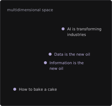
To generate them, we need an embedding model. It's a specialized neural network, often derived from the same architectures behind modern LLMs, trained to represent text as coordinates in a multidimensional space.
To do that, it has been exposed to billions of words, sentences and documents, gradually learning the relationships between concepts. As a result, concepts that share similar meanings tend to end up close together, while unrelated ones are placed further apart.
If we take a closer look [0.0125, -0.3412, 0.8912, 0.0045, ...], we can identify two key properties that define both its expressive power and its memory footprint.
The first is the individual number itself 0.0125. Each value in the array is typically a 32-bit floating point number (float32), which means it takes exactly 4 bytes of memory per value.
The second is the dimension of the array, the number of values it contains. This is fixed for a given model and is often referred to as the embedding dimension. In general, higher dimensionality allows the model to capture more subtle semantic nuances, at the cost of increased storage and computation.
This is where the exploration really begins.
Once you start working with embeddings on real data, questions start to arise:
- What is a meaningful sample size?
- How does memory footprint influence this choice?
- Which languages should be supported? Just English, or the full catalog?
- What about storage, production and hardware constraints?
- Do we need to care about text length?
- Which embedding model should I use?
And so on.
When I build software, my approach is always local-first. Whether it's just a prototype or something closer to a production-grade system, it should be able to run on my machine with as little friction as possible. For this reason, one of the first things I focused on was the choice of the embedding model. It had to run comfortably on my local hardware, which immediately influenced a chain of decisions: sample size, memory footprint and even language support all became downstream consequences of that choice.
My hardware concerns were relatively limited, being an avid gamer. We'll get back to that later.
At this point, I recalled a demo and its related blog post shared by Loreto and Francesco, co-founders and managers where I work:
- Quantized Retrieval
- Binary and Scalar Embedding Quantization for Significantly Faster & Cheaper Retrieval
As a side note about antirez: the word "quantization" should immediately remind you of what he's doing with ds4. If you don't know it yet, it's worth taking a look.
The demo and the blog post describe a semantic retrieval system built over 41 million Wikipedia texts. You type a sentence and within milliseconds it surfaces the most semantically similar passages.
What's striking is not just the speed, but how much accuracy is preserved while drastically reducing memory footprint through quantization.
Quantizing an embedding means reducing the precision used to represent each number in the vector. Do we really need that many decimal places when all we care about is whether two vectors are close or far apart?
In most cases, the answer is no. We can safely round these values in a controlled way, trading a small amount of precision for a massive gain in space. The model used in the demo (mxbai-embed-large-v1, an open-source embedding model) produces embeddings with 1024 dimensions.
Stored as float32, each vector takes:
1024 * 4 bytes = 4096 bytes per vector
Now consider what happens when we want to retrieve the most similar vector to a query. We need to compare it against every single vector in the dataset. For this to be fast, everything has to live in memory, ideally RAM.
With 41 million vectors:
41M * 4096 bytes ≈ 168 GB of RAM
This is exactly where quantization comes in and it does so at two different levels:
- Scalar quantization
(int8), eachfloat32value (4 bytes, ~7 decimal digits of precision) is mapped to an integer between -128 and +127 (1 byte, 256 discrete levels).
float32: 0.7392473... → int8: 94
float32: -0.2481552... → int8: -32

1024 dimensions * 1 byte = 1024 bytes per vector (4x smaller)
41M * 1024 bytes ≈ 42 GB
- Binary quantization, each value is reduced to a single bit, positive becomes 1, negative becomes 0. The most extreme form of rounding.
float32: 0.7392... → 1 (positive)
float32: -0.2481... → 0 (negative)

1024 dimensions * 1 bit = 128 bytes per vector (32x smaller)
41M * 128 bytes ≈ 5.2 GB
At this point, you would expect that compressing vectors by up to 32x would completely destroy retrieval quality. This is where the numbers become surprising:
|                          | float32 (original) | int8 (4x compression) | binary (32x compression) |
|--------------------------|--------------------|------------------------|---------------------------|
| Space per vector         | 4096 bytes         | 1024 bytes             | 128 bytes                 |
| Space for 41M vectors    | ~168 GB            | ~42 GB                 | ~5.2 GB                   |
| Retrieval speed          | 1x (baseline)      | ~3.7x                  | ~25x                      |
| **Quality preserved**    | **100%**           | **~99.3%**             | **~96%**                  |
32x compression. ~4% loss in ranking quality. ~25x faster retrieval. From 168 GB of RAM down to 5.2 GB.
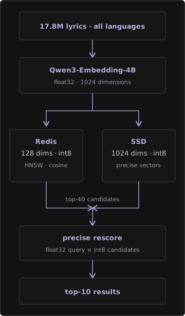
The demo and blog post propose combining both levels into a two-stage architecture that almost fully recovers the precision lost in compression:
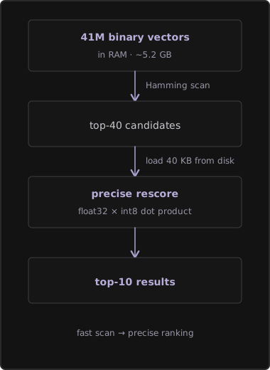
The first stage uses the most compressed representation (binary) to eliminate 99.99% of irrelevant documents. The second stage retrieves only the surviving 40 candidates in their higher-precision int8 form and re-ranks them.
The combined result: final retrieval quality climbs back to ~99%. Close to full float32 quality, while using 1/30 of the memory and 1/25 of the compute time.
With that recipe in hand, I settled on ~18 million lyrics spanning 100+ languages (~53% English, ~47% other languages).
Running the same math:
17.8M × 4096 bytes (float32) ≈ 73 GB
17.8M × 1024 bytes (int8)    ≈ 18 GB
17.8M × 128 bytes  (binary)  ≈ 2.3 GB
2.3 GB of RAM for the fast index. 18 GB on SSD for the precise rescore.
My MacBook Air M4 has 16 GB of RAM and a 512 GB SSD. It fits.
But I didn't want to simply replicate the demo. I wanted to explore something closer to a production backend system and this is where Salvatore's work became relevant again: Redis as the first-stage engine.
The Hugging Face demo uses Faiss, a C++ library by Meta for vector similarity search. Every instance of your application loads its own copy of the index. There's no shared state, no API boundary, no familiar infrastructure.
Redis, on the other hand, is a service and since version 8.0 it supports vector search natively.
There's a catch, though. Redis actually exposes vectors through two different engines: the query engine's vector index (FT.CREATE / FT.SEARCH) and Vector Sets (VADD / VSIM), the data type Salvatore designed himself. Neither one exposes Hamming distance as a retrieval metric.
The query engine ranks with geometric metrics (L2, IP and COSINE) over numerical types like float16, float32, float64, bfloat16, int8 and uint8. Vector Sets can store vectors with binary quantization (BIN, 32x smaller, the same bit-level trick the HF demo leans on), but even there the ranking is cosine, not Hamming.
So the HF demo's exact recipe can't be reproduced one-to-one on Redis. I needed an alternative that would:
- Fit in the same ~128 bytes per vector (to keep RAM at ~2.3 GB)
- Work with Redis's supported distance metrics
- Preserve retrieval quality
🪆 Matryoshka.
Certain embedding models are trained so that the first N dimensions of the vector already carry most of the semantic information. You can truncate a 1024-dimensional vector to its first 128 dimensions and still get a meaningful representation.
Think of it like a Russian nesting doll: the smaller version inside still looks like the original.
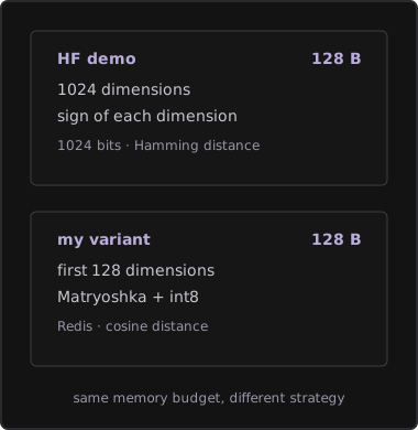
Same memory budget (128 bytes per vector), different compression strategy. The HF demo discards magnitude information (keeping only the sign). My variant discards the less-important dimensions (keeping the most informative ones, thanks to Matryoshka training).
As mentioned, the HF demo uses mxbai-embed-large-v1, an English-only model with a 512-token context window. For my dataset this is limiting, lyrics exceed 512 tokens and are in multiple languages.
I ended up choosing Qwen3-Embedding-4B:
- 32K token context window (no lyric will ever be truncated)
- Supports 100+ languages
- Matryoshka: natively 2560-dim, but I ask for 1024 (
mxbai's size), then truncate to 128
The trade-off here is speed. 4B parameters means ~12x slower than the 335M parameter mxbai. But embedding generation is a one-time batch job and do you recall I'm an avid gamer? I have a GPU that can handle it, my desktop's RTX 4070. After that, searches are instantaneous regardless of model size (I know we still need to embed the queries...).
The pipeline looks like this:
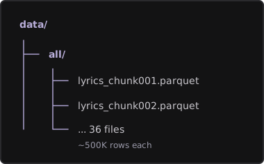
Before running any embedding, I needed the raw lyrics in a format suitable for batch processing on the desktop GPU.
At this scale, format matters. I opted for Parquet, a columnar and compressed format where each row carries:
- The ID
- Lyrics
- Track name
- Artist name
- Language
The full dataset sits at ~10 GB on disk, as CSV it would be 35-40 GB.
Being columnar also means selective reads. When I only need IDs and language codes (for example, to count how many English tracks I have), Parquet skips the lyrics entirely. This turned out useful more than once.
With the data on disk, the next step was straightforward. I copied the files to an external drive and plugged it into the desktop.
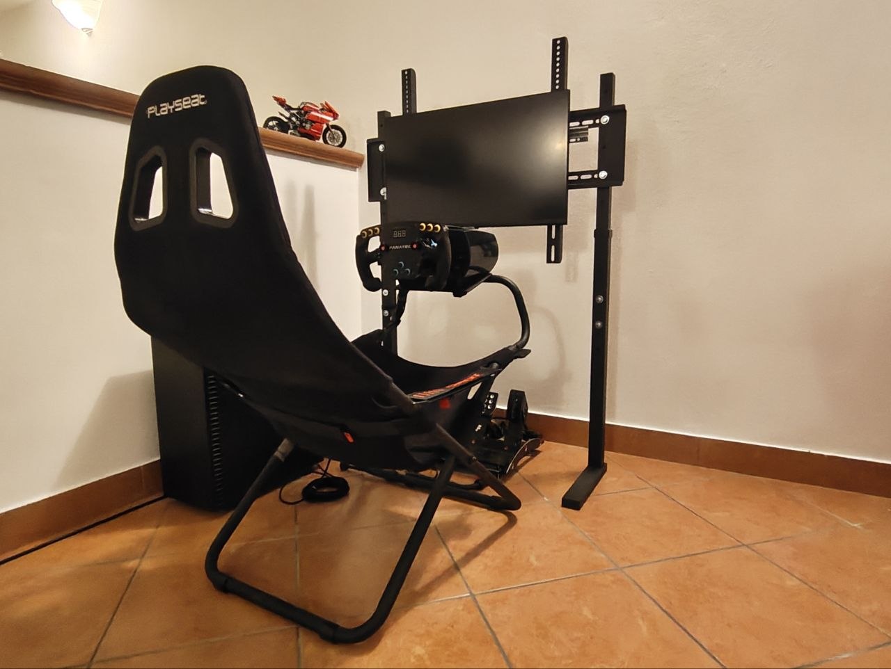
As you can tell from the rig photo, it is ready for time attacks on any F1 circuit, but completely unprepared for computing embeddings. In addition to the racing wheel, my only input device was a Rii Mini i8, a tiny wireless keyboard with a built-in trackpad which made typing Windows PowerShell commands a nightmare.
With that infernal contraption, I had to set up a python environment from scratch, starting with a virtual environment and the key project dependency: PyTorch.
PyTorch is Meta's open-source framework for GPU-accelerated matrix operations. A neural network like Qwen3-Embedding-4B is, at its core, a sequence of matrix multiplications. When you feed it a text:
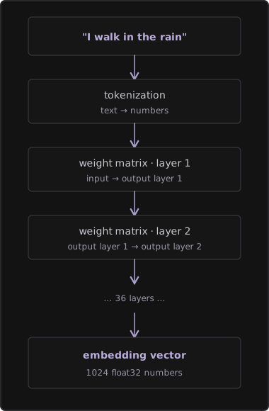
Each layer is a large matrix multiplication. Qwen3-4B has 4 billion parameters, 4 billion numbers spread across these matrices.
My RTX 4070 has 5,888 CUDA cores. They're simple cores, but thousands of them work in parallel. This makes GPUs roughly 50–100x faster than a CPU for this kind of workload.
The other project dependencies were minimal:
sentence-transformerswraps the model loading and inference into a clean API.Qwen3-Embedding-4Bis available as a sentence-transformers model, so encoding text becomes a single function callpyarrowreads Parquet files. Without it, I can't access the lyricsnumpyhandles the memory-mapped files and the quantization math
A quick sanity check on PowerShell before launching:
python -c "import torch; print(f'CUDA: {torch.cuda.is_available()}'); print(f'GPU: {torch.cuda.get_device_name(0)}')"
CUDA: True
GPU: NVIDIA GeForce RTX 4070
With everything in place, the embedding script itself is surprisingly compact. The same script handles model loading, encoding and persistence to disk. It starts with four lines to load the model, specifying which dimension to truncate to (remember, Matryoshka lets you do this) and which device to run on:
from sentence_transformers import SentenceTransformer

model = SentenceTransformer(
    "Qwen/Qwen3-Embedding-4B",
    truncate_dim=1024,          # Matryoshka: 2560 → 1024
    device="cuda",              # RTX 4070
    trust_remote_code=True,
)
For each batch of lyrics, encoding is a one-liner:
embeddings = model.encode(
    batch_texts,                # list of lyrics
    normalize_embeddings=True,  # L2 normalize → cosine similarity becomes dot product
)
But where do those vectors go? 17.8 million of them at 1024 floats each means ~73 GB. That clearly won't fit in RAM. This is where memory-mapped files come in — the same mechanism the operating system uses for virtual memory. You allocate a file on disk with a fixed shape, and numpy lets you write to it as if it were an in-memory array:
import numpy as np

# Allocate the file on disk with the final shape — 0 bytes in RAM
mmap = np.memmap(
    "embeddings_float32_1024.mmap",
    dtype=np.float32,
    mode="w+",
    shape=(17_832_497, 1024),  # 17.8M × 1024 ≈ 73 GB on disk
)

# Write batch by batch, directly to disk
mmap[current_row:current_row + batch_size] = embeddings
The script processes all 17.8 million lyrics in batches of 32, writing each batch directly to disk. Progress is tracked in a text file so that if it crashes at 3 AM, I can relaunch and it picks up where it left off.
Once all embeddings are on disk, quantization is just linear algebra. Mapping float32 values into 256 discrete levels in code:
# Compute the range for each dimension across the entire dataset
dim_min = float32_mmap.min(axis=0)  # minimum across all 17.8M vectors, per dimension
dim_max = float32_mmap.max(axis=0)  # maximum across all 17.8M vectors, per dimension

# Linearly map each float to the range [-128, 127]
scale = 255.0 / (dim_max - dim_min)
int8_values = ((float32_values - dim_min) * scale - 128).astype(np.int8)
As described in the HF blog post, computing min/max over the entire dataset ensures each dimension uses its full 256-level range optimally. The result: embeddings_int8_1024.mmap (~18 GB), ready for the rescore stage.
The same operation, applied to the first 128 dimensions only (the Matryoshka-truncated version), produces the one that goes into Redis: embeddings_int8_128.mmap (~2.3 GB).
Time to go to sleep and let the GPU do some math. See you tomorrow morning, hopefully we don't wake up dead.
CJ: How the hell do you wake up dead?
Mahalik: Cause' you're alive when you go to sleep.
CJ: So you're telling me you can go to bed dead and wake up alive?
Mahalik: You can't go to bed dead! That shit would've been redundant.
CJ: No it would'nt cause' you can go to bed and not be dead, and you can die and not be in the bed.
Mahalik: but you are in the bed. That's how you wake up dead in the first place fool!
CJ: Damn! That's some quantum shit right there man! You should be teaching classes!